Earth Normal Maps from NASA Elevation Data
In this post, I’ll describe how to convert a raw NASA height map of earth into a normal map, which can then be used for normal mapping 3D models.
It Starts With Height
Let’s start with downloading the raw data from NASA. For this example, I will use the .png file they provide.
Open this file in Photoshop, or in any other image editing tool and you will see a projection of the world, already laid out so that the texture coordinates will fit the most common way of texturing a sphere. The image is grayscale, and 8 bit, which means it can show 256 different levels of height. Because elevation begins at sea level, we can assume that 0 brightness means 0 height, and 100% brightness represents the highest elevation (8800m or so). And indeed, the oceans show up with 0% brightness, and the Himalayas appear pretty bright.
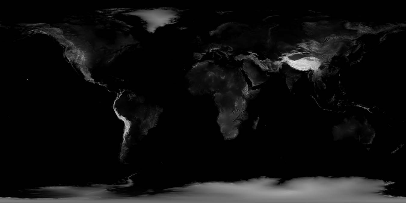
This is how the orignal grayscale image should look like
To calculate the normals, we are not super-interested in getting the actual height of a point on the map, but we’re interested in the gradient.
A bit of Background: Why are we Interested in the Gradient?
The gradient refers to change in height between neighbouring points.
Let’s do a ridiculous thought experiment: Imagine you stand on a snowboard, on a mountain. That’s your current point. The next point you are interested in is somewhere ahead of you, and below you. Now point your snowboard straight down the slope, to this point. While you slide down, make sure to keep your body perpendicular to your snowboard. Congratulations, you have just transformed your body into a 2D normal!

Now, repeat this with a pair of skis. Here, before you even start off, cross your skis so that they are at a 90 degree angle. You will notice that the skis will follow the incline of a different slope for each leg. Nevermind, defy gravity, and attempt to keep your body perpendicular to both skis. With this, you have just transformed your body into a 3D normal.
Because of such a relationship between two slopes and the normal, the shader can calculate the current normal for any textured fragment, reading the slope from the red and green channel of the normal map.
How this works in detail is best described in Mathematics for 3D Programming by Eric Lengyel, and would be enough material for a separate post. It’s important to note, however, that there are two gradients we need to calculate, one in x direction and one in y direction.
Calculate Gradients
One of the ways to calculate the gradient between neighbouring pixels is using Sobel operators. The Sobel operator is a simple convolution kernel, and can easily be applied in Photoshop, using the “Custom Filter” option.
To get the gradient in x, we use this Sobel operator:
$$ \begin{equation*} S_{x} = \begin{bmatrix} 1 & 0 & -1 \\ 2 & 0 & -2 \\ 1 & 0 & -1 \end{bmatrix} \end{equation*} $$
To get the gradient in y, we use this Sobel operator:
$$ \begin{equation*} S_{y} = \begin{bmatrix} 1 & 2 & 1 \\ 0 & 0 & 0 \\ -1 & -2 & -1 \end{bmatrix} \end{equation*} $$
I’ve prepared two convolution kernel files, the first one applies the Sobel operation in x direction, the other applies it in ydirection.
Step by Step
- First, convert the grayscale image to RGB colours, so that we can store the results of the Sobel operations in separate channels. We’re not terribly interested in the blue channel, so:
- In the “Channel” view, select the Blue channel, select all, then clear it and fill it with 100% brightness.
- Then select the Red channel. You should see the initial grayscale image height map. Apply the
sobel_dxkernel to this red channel. “Filter” → “Other” → “Custom” → “Load” →sobel_dx.acf→ “Apply”. The height map should transform into something more like a brighter relief map, but still be grayscale. - Then select the Green channel, and repeat the steps from 3., but with the
sobel_dykernel. - Then, in channel view, select RGB - you should see something looking like this:
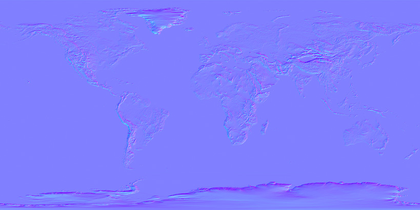
Use the color sampler to find out the color value of a pixel somewhere in the ocean. If it comes back with value [128,128,255] it most probably worked.
I recommend saving the file as PNG or any other non-destructive format, because JPEG, for example, will distort your normal map data when compressing the image.
Here are some final results:
- Normal Map Earth, (16384x8192), TIFF 16 bit Download (~146 MB)
- Normal Map Earth, (8192x4096), PNG 8 bit Download (~24 MB)
Tagged:
RSS:
Find out first about new posts by subscribing to the RSS Feed
Further Posts:
- Vulkan Video Decode: First Frames
- C++20 Coroutines Driving a Job System
- Vulkan Render-Queues and how they Sync
- Rendergraphs and how to implement one
- Implementing Bitonic Merge Sort in Vulkan Compute
- Callbacks and Hot-Reloading Reloaded: Bring your own PLT
- Callbacks and Hot-Reloading: Must JMP through extra hoops
- How far back should the screen go?
- Using ofxPlaylist
- Flat Shading using legacy GLSL on OSX